How Window Functions Work

What are Window Functions?

Window functions create a new column based on calculations performed on a subset or “window” of the data. This window starts at the first row on a particular column and increases in size unless you constrain the size of the window.

SELECT 'Day', 'Mile Driving',
SUM('Miles Driving') OVER(ORDER BY 'Day') AS 'Running Total'
FROM 'Running total mileage visual';

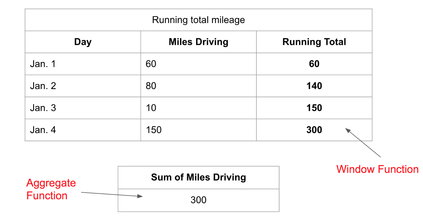
Here we can see it perform an aggregation of what is in side of the window. The window grows each row and so it aggregates more and more of the data giving you a running aggregation, in this case a running total.

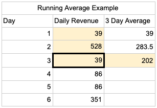
If we constrain the window to be 3 rows tall we can get a 3 day running average.

SELECT 'Day', 'Daily Revenue',
AVG('Daily Revenue') OVER(ORDER BY 'Day' ROWS 2 PRECEDING)
AS '3 Day Average' FROM 'Running Average Example';

The window still starts as a single row, then it grows to its fixed size and then the whole window shifts along with it.

Window functions also work on partitioned data (grouped data). It first sorts the data then applies the aggregate function on those groups, putting the result in the new column for each row in that group.

Below, you can see an example of this calculating the total revenue a business makes on the weekend vs the rest of the week.

SELECT 'Day', 'Weekend', 'Daily Revenue',
SUM('Daily Revenue') OVER(PARTITION BY 'Weekend') AS 'Total'
FROM 'Partitioned Total Example';

Window functions are very similar to aggregation functions, in fact every window function applies an aggregation within it. The difference are:

Output:

• Aggregations produce a single row of output for rows the aggregation was applied to
• Window functions produce a new column of data that is the same number of rows as the data it was applied to.

Subsetting the data:

• Aggregations are applied to data that is grouped categorically or across the whole data set.
• Window functions are applied to the data within a window. The window can scale in size with each row, be constrained to a specific amount of rows, or can fit groups.

Let’s look at the first example above if we applied an aggregation instead of a window function to it.

Window Function:

SELECT 'Day', 'Mile Driving',
SUM('Miles Driving') OVER(ORDER BY 'Day') AS 'Running Total'
FROM 'Running total mileage visual';

Aggregate:

SELECT SUM('Miles Driving') AS 'Sum of Miles Driving'
FROM 'Running total mileage visual';

Window Functions can be used to create running totals, moving averages and much more. The three main keywords to create a Window Function are:

• OVER
• PARTITION BY
• ORDER BY

OVER - Indicates the beginning of a Window Function, this causes the results of the aggregation to be added as a column to the output table.

PARTITION BY - Creates groups of data in the table, that the aggregation will be performed on.

ORDER BY - Sorts the data based on the given column.

Now, let’s look at these keywords within a full query.

Syntax

SELECT '(Optional: The data you want to select)',
[aggregate function]'(The column to perform the aggregate function on)'
OVER(Optional: PARTITION BY and/or ORDER BY)
AS '(Descriptive name)' FROM '(corresponding table)';

Going back to the first example the query would look like:

SELECT 'Date', 'Miles Driving',
SUM('Miles Driving') OVER(ORDER BY Date) AS 'Running Total'
FROM 'Running Total Mileage';

The SUM keyword shows that the query is looking for the SUM of the “Miles Driving” column, shown OVER the whole table, ORDERed BY the date the mileage will occur.

Example

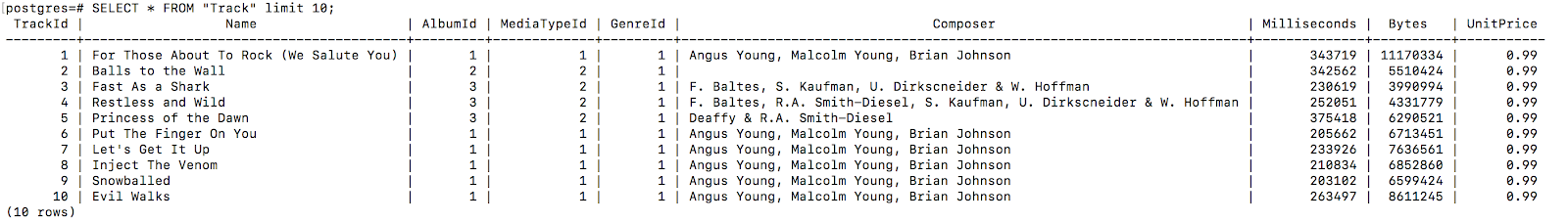
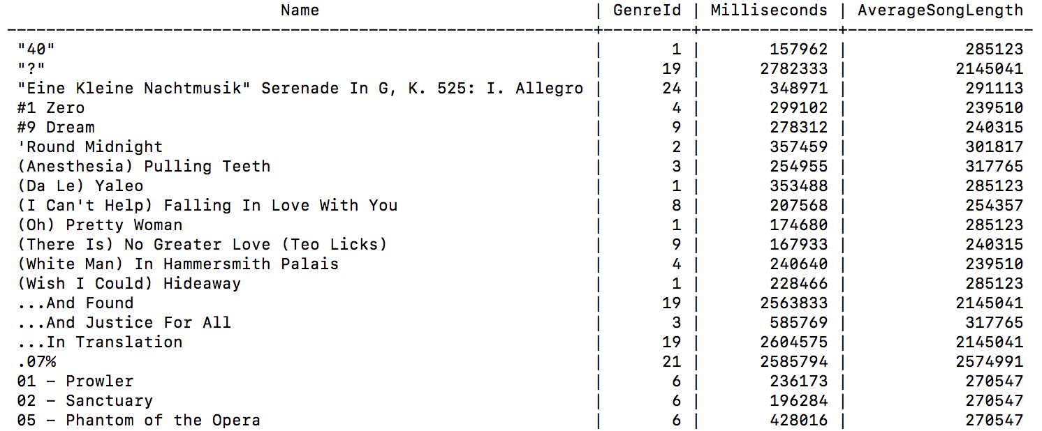
The example below uses the Chinook database with PostgreSQL 11. The “Track” table in the Chinook database is a large, informational table on many different songs by many different artists:

If you wanted to create a column displaying the average song length you can do so like:

SELECT Track.Name, Track.Milliseconds
AVG(Track.Milliseconds) OVER() AS 'AverageSongLength'
FROM 'Track' LIMIT 20;

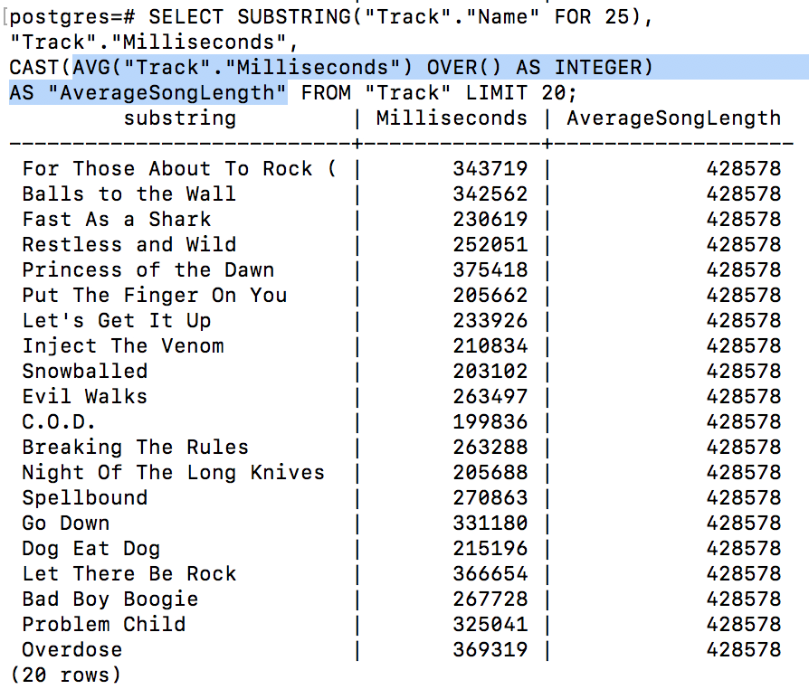
You can see the “AverageSongLength” is stored in the last column and is the same for every row. This can help you visualize and compare songs that are longer or shorter than the “AverageSongLength”.

Organizing with Window Functions

Using ROWS

The window can also be given specific size dimensions using the ROWS keyword. You can specify the number or rows you want the window to be with the keywords:

PRECEDING - define the number of rows before the current row to include FOLLOWING - define the number of rows after the current row to include

Syntax

SELECT '(The data you want to select)',
[aggregate function]'(The column to perform the aggregate function on)'
OVER(ROWS [# of rows you want to aggregate - 1] PRECEDING/FOLLOWING)
AS '(descriptive name)'
FROM '(appropriate table)';

Example

SELECT *,
AVG('Daily Revenue')
OVER(ROWS 2 PRECEDING)
AS '3 Day Average'
FROM 'Running Average Example'

SELECT *,
AVG('Daily Revenue')
OVER(ROWS 2 FOLLOWING)
AS '3 Day Average'
FROM 'Running Average Example'

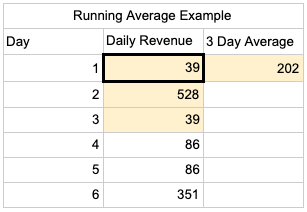
You use one less than the days you would like to average because the query executes the aggregate function of the current row and the number of specified preceding or following rows. This allows you to create moving averages, which are great for showing more general trends in data.

Using PARTITION BY

PARTITION BY is used to group the data before performing an aggregate function so that the aggregation runs on each category independently.

Syntax

SELECT '(The data you want to select)',
[aggregate function]'(The column to perform the aggregate function on)'
OVER(PARTITION BY [category to group by]) AS '(descriptive name)'
FROM '(appropriate table)';

Example

If you wanted to compare the average length of a song by the genre of the song, you can run the same query as above just adding the partition:

SELECT Track.Name, Track.Milliseconds
AVG(Track.Milliseconds) OVER(PARTITION BY Track.GenreId)
AS 'AverageSongLength'
FROM 'Track' ORDER BY Track.Name ASC LIMIT 20;

You can see that the average song length from the first example is not the same average song length for all songs grouped by their genres.

Using ORDER BY

Traditionally, ORDER BY is called on the whole table(as seen above) and will sort the table by the given column. There are two circumstances ORDER BY can be used in:

1. Without PARTITION BY: ORDER BY will sort like the traditional ORDER BY while also causing the aggregate function to be applied incrementally, providing a new, recalculated value for every row in the table.(first example below)
2. With PARTITION BY: ORDER BY will sort each partition individually by the given column and cause the aggregate function to be applied incrementally for each partition.

Example

If you had the data for the daily steps taken by an individual:

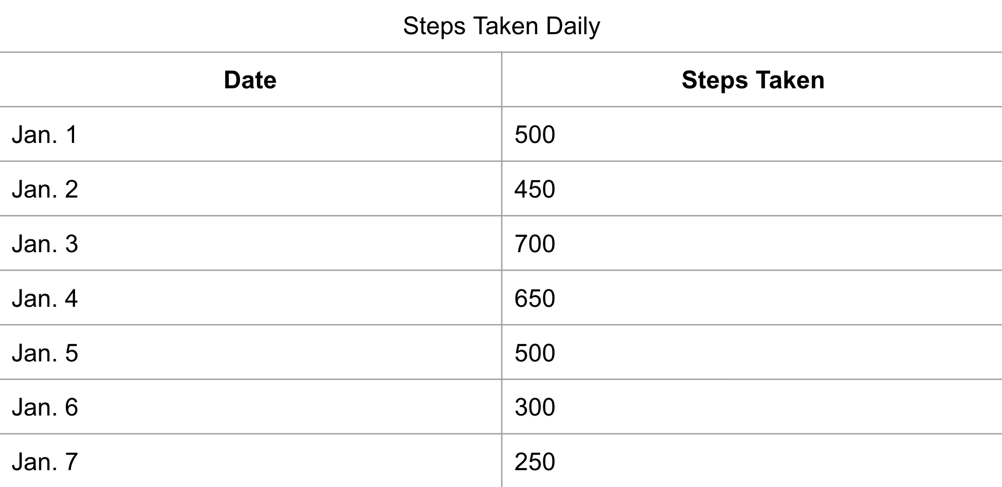
You could begin to find the average number of steps someone has taken in a week to determine their weekly activity levels:

SELECT 'Date', 'Steps Taken',
AVG('Steps Taken') OVER(ORDER BY Date)
AS 'Average Steps Taken'
FROM 'Steps Taken Daily';

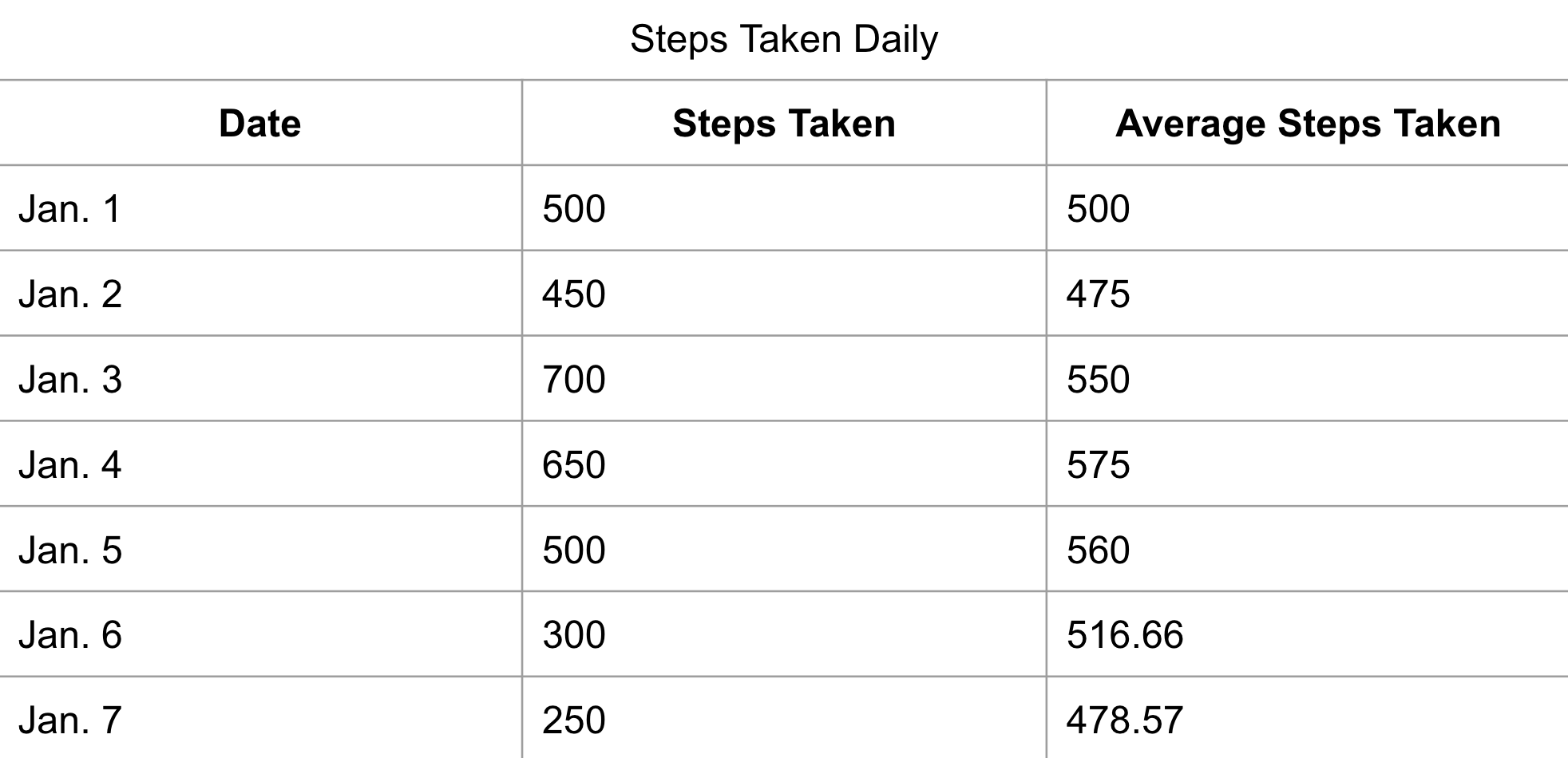
You should notice that, since ORDER BY was used, the AVG function is taken as the “running average”. So the AVG is recalculated in every row.

We could also use PARTITION BY with ORDER BY, implementing a weekend indicator, to separate the weekday running average from weekend running average:

SELECT 'Date', 'Weekend', 'Steps Taken',
AVG('Steps Taken') OVER(PARTITION BY 'Weekend' ORDER BY Date)
AS 'Average Steps Taken' FROM 'Steps Taken Daily';

Looking at the data above, you can see that when used with PARTITION BY, ORDER BY still creates a “running average”. Again, note that Window Functions do not return two new rows just displaying the average steps from during the week and on the weekend, the running average is displayed as a new column on the end of the data.

Summary

• A window function does not cause rows to become grouped into a single output row, it creates a whole output column.
• A window function can be broken into groups and organized easily with keywords like: PARTITION BY and ORDER BY.
  • PARTITION BY- Divides the aggregate function results between different groupings of data.
  • ORDER BY- Organize the data being worked on by the aggregate functions and create running calculations

References

https://mode.com/sql-tutorial/sql-window-functions/

https://www.postgresql.org/docs/9.1/tutorial-window.html

Written by: Blake Barnhill
Reviewed by: Matt David , Matthew Layne